
My updates to this blog have been quite sporadic of late, as life has been having a tendency of getting in the way. However, I could not let this week go by without noting this year’s Nobel Prize for Physics, particularly since it involves something near and dear to me: the ephemeral elementary particles known as neutrinos. (I’ve dropped hints in the past of a mega-post on the topic that has taken on a life of its own as I’ve continued to find new material to add. Much of this post will summarize material from that work.)
On Tuesday, the Royal Swedish Academy of Sciences announced that the 2015 Nobel Prize in Physics was being awarded to Takaaki Kajita (of the Super-Kamiokande Collaboration in Japan) and Arthur B. McDonald (of the Sudbury Neutrino Observatory Collaboration in Canada) “for the discovery of neutrino oscillations, which shows that neutrinos have mass.”
This is all about neutrino oscillation, the changing of a neutrino from one “flavour” to another over time. This ability had for a few decades been considered a potential explanation for something called the solar neutrino problem, which I will describe shortly. However, in order for neutrino oscillation to take place, it would mean that neutrinos would have to have some mass, despite being treated as massless by the Standard Model of particle physics for decades. (In an Appendix at the bottom of this post, I work through the mathematics from which this requirement is derived.) The work of the teams led by Kajita and McDonald demonstrated that neutrino oscillation does indeed take place, thus neutrinos do have mass (albeit a VERY tiny mass).
Background
In 1914, James Chadwick had encountered a problem. The energy spectrum of beta particles (high energy electrons or positrons, depending upon the particular reaction) emitted by certain radioactive decays was continuous, but should have had a fixed value. This was problematic, as it represented a potential breakdown of the law of conservation of energy. (Conservation of angular momentum was also at stake, given the spins of the particles involved, but spin wasn’t really well-understood at the time.)
On December 4, 1930, Wolfgang Pauli (of “Pauli Exclusion Principle” fame) wrote an open letter to his colleagues attending a conference in Tübingen, Germany, opening with the rather humorous salutation “Liebe Radioaktive Damen und Herren” (“Dear Radioactive Ladies and Gentlemen”), in which he proposed a possible mechanism for saving conservation of energy in β-decays. So uncertain and tentative was the esteemed Dr. Pauli of his idea that he was not yet ready to submit his proposal for publication in a journal.

A stylized pseudo-Feynman diagram showing the Standard Model concept of beta decay: one down quark in the neutron decays to an up quark and a W- boson, which then decays to an electron and an anti-neutrino. (Illustration by the author.)
In the letter, Pauli proposed the existence of an electrically-neutral, massless (or at least very light), weakly interacting (thus evading detection) fermion emitted by β-decay along with the electron, carrying with it the “missing” energy, thus balancing out the energy and spin of the reaction. He dubbed this new particle the “neutron.” However, since his idea did not gain much traction at first, that name was snatched by James Chadwick upon his discovery in 1932 of the neutral baryon which now bears the name. To clear up the confusion, Enrico Fermi coined the name “neutrino” (“little neutral one”) for Pauli’s particle in 1933, and in 1934 incorporated it into a more complete theory for β-decay, his theory of the weak nuclear force.
Pauli sometimes expressed regret for ever coming up this particle, since he felt it would be nearly impossible to experimentally detect. The weak nuclear force is well-named, and because of that weakness (or, more specifically, due to the massiveness of the W and Z bosons which mediate the force), it has an exceedingly short range. For an interaction to take place, a neutrino must pretty much strike a nucleon dead-on. Given how little the volume of a given atom is taken by nucleons, it is then no small wonder that that the mean free path (the average distance an individual particle will travel before interacting) of a neutrino in solid lead is a few light years. On the other hand, neutrinos are the second most abundant elementary particle in the universe, surpassed only by photons. In any given seconds, trillions of them are passing right through your body. So, detecting neutrinos boils down to having a large eough volume of detection medium, and a way of filtering out other particles or radiation which might generate false-positive results, preferably by locating the detector deep underground.
It took a few decades, but neutrinos were finally detected in 1956 by Fred Reines and Clyde Cowan of Los Alamos National Lab in a series of experiments at the Savannah River nuclear reactor and the Hanford nuclear reactor. It seems only fitting that the effort to detect these ephemeral particles was known as Project Poltergeist.
- F. Reines and C. L. Cowan, Jr. “Detection of the Free Neutrino” Phys. Rev. 92, 830 (1953)
- C.L. Cowan, Jr., F. Reines, F.B. Harrison, H.W. Kruse and A.D. McGuire,”Detection of the Free Neutrino: A Confirmation”, Science 124, 103 (1956). doi: 10.1126/science.124.3212.103
- Frederick Reines and Clyde L. Cowan, Jr., “The Neutrino”, Nature 178, 446 (1956). doi: 10.1038/178446a0
- “Neutrino Physics”, Frederick Reines and Clyde L. Cowan, Jr., Physics Today 10, no. 8, p.12 (1957). doi: 10.1063/1.3060455
The Problem
In 1968, Ray Davis and John N. Bahcall were running an experiment in the Homestake gold mine in South Dakota studying solar neutrinos (well, technically anti-neutrinos, but that isn’t important for the purposes of this discussion). But something was amiss. Davis’ chlorine-based neutrino detector was only picking up approximately one-third of the solar neutrino flux predicted by Bahcall’s models. Either something was wrong with the detector, or with Bahcall’s calculations, or a large portion of the neutrinos from the sun were going missing. This issue came to be known as the solar neutrino problem, and it vexed physicists. Numerous measurements performed by various teams over the ensuing years replicated the result. Researchers specializing in the physics of the interior of the sun poured over Bahcall’s model, but could find nothing wrong with his calculations. The neutrinos from the sun WERE going missing.
- Cleveland, B. T. et al. (1998). “Measurement of the solar electron neutrino flux with the Homestake chlorine detector”. Astrophysical Journal 496: 505–526. Bibcode 1998ApJ…496..505C. doi: 10.1086/305343
- Davis, R. Jr. “Search for Neutrinos from the Sun”, Brookhaven National Laboratory (BNL), United States Department of Energy (through predecessor agency theAtomic Energy Commission, (1968).
- Davis, R. Jr. & J.C. Evans, Jr. “Report on the Brookhaven Solar Neutrino Experiment”, Brookhaven National Laboratory (BNL), (September 22, 1976).
- Davis, R. Jr., Evans, J. C. & B. T. Cleveland. “Solar Neutrino Problem”, Brookhaven National Laboratory (BNL), (April 28, 1978).
- Davis, R. Jr., Cleveland, B. T. & J. K. Rowley. “Variations in the Solar Neutrino Flux”, Department of Astronomy and Astrophysics at University of Pennsylvania, Los Alamos National Laboratory (LANL), Brookhaven National Laboratory (BNL), (August 2, 1987).
The Solution
It actually didn’t take long for a potential solution to be developed. Recall that the detector in the Homestake mine was chlorine-based. It consisted essentially of a large tank of chlorine-based cleaning fluid. An anti-neutrino from the sun would strike a Chlorine-37 nucleus, converting a neutron into a proton and an electron, resulting in the generation of Argon-37 which could be separated out and measured. The problem, however, is that this reaction is only sensitive to electron anti-neutrinos.
You see, there are three types, or “flavours,” of neutrinos, each associated with one of the three types of charged leptons. Electron neutrinos are produced or absorbed in weak interactions involving electrons, muon neutrinos are associated with interactions involving muons, and tau neutrinos are associated with interactions involving tau leptons.
In 1957, Bruno Pontecorvo, an Italian physicist living in the USSR (and the same physicist who came up with the scheme of electron and muon lepton numbers), formulated a theory of neutrino “oscillations.” He speculated that neutrinos and antineutrinos might be able to oscillate back and forth between each other. This has never been observed, but in 1962, Ziro Maki, Masami Nakagawa, and Shoichi Sakata introduced what is now known as the Pontecorvo–Maki–Nakagawa–Sakata (or PMNS) matrix to extend Pontecorvo’s idea to oscillation between neutrino weak flavours. This was followed by a subsequent paper by Pontecorvo in 1967 elaborating upon the idea.
Here are the basics of how neutrino mixing works. Consider two waves. It doesn’t matter what they are waves of, we are primarily dealing with the mathematical properties of waves in general. What happens if we combine or superimpose the waves? If the two waves have the same frequency, then the combined wave will have that same single constant frequency (perhaps phase shifted and with amplitudes enhanced or diminished due to phase differences between the two waves). However, if the two waves have slightly different frequencies, then they will interfere with one another such that the combined wave will vary in frequency.
Any given neutrino does not have a pure flavour, which is to say, it is not an electron neutrino, a muon neutrino, or a tau neutrino, until it is measured to be one or another. The neutrino is a superposition of all three (sort of – see details in the Appendix below). The quantum wave representing each neutrino type has a different frequency proportional to its mass. Because the probability of measuring each neutrino type is proportional to the square of its wave function, and because of interference between these three frequencies, the probability of which type of neutrino would be detected oscillates at a rate proportional to the difference between the squares of the masses. Consequently, neutrino oscillation will only occur if the masses of the three neutrino types are different, which means that they cannot all be zero. (This leaves open the possibility that the lightest of the neutrino species could have zero mass, provided that the other two have two distinct non-zero masses, but physicists suspect this is not the case.)
As pointed out above, there was one catch with Pontecorvo’s scheme. Oscillation would only occur if neutrinos possess mass (with the differences in the squares of the masses determining the rate of the oscillation), and neutrinos were thought at the time to be massless since neutrinos are not able to couple to the Higgs field.
- B. Pontecorvo (1957). “Mesonium and anti-mesonium”. Zh. Eksp. Teor. Fiz. 33: 549–551. reproduced and translated in Sov. Phys. JETP 6: 429. 1958. Bibcode 1958JETP….6..429P
- B. Pontecorvo (1967). “Neutrino Experiments and the Problem of Conservation of Leptonic Charge”. Zh. Eksp. Teor. Fiz. 53: 1717. reproduced and translated in Sov. Phys. JETP 26: 984. 1968. Bibcode 1968JETP…26..984P
- Z. Maki, M. Nakagawa, and S. Sakata (1962). “Remarks on the Unified Model of Elementary Particles”. Progress of Theoretical Physics 28: 870. Bibcode 1962PThPh..28..870M. doi: 10.1143/PTP.28.870
The Evidence
And now we come to the experimental validation of the neutrino oscillation idea.
At the Neutrino ’98 conference in Japan, a group of scientists from the Super-Kamiokande experiment presented startling results from their study of muon neutrinos formed by the interaction of cosmic rays with the upper atmosphere. They found that the flux of such neutrinos coming from underneath (having passed through the bulk of the earth, something that neutrinos do quite easily) was lower than those coming from overhead, implying a distance relationship in the neutrino flux. Pontecorvo’s old oscillation model started cropping up again in attempts to interpret the result, along with suggestions that neutrino oscillation could be the solution to the solar neutrino problem. The previously outlandish idea that neutrinos had mass (albeit a minuscule amount) was starting to gain traction.
- Fukuda, Y., et al (1998). “Measurements of the Solar Neutrino Flux from Super-Kamiokande’s First 300 Days”. Physical Review Letters 81 (6): 1158–1162. arXiv: hep-ex/9805021. Bibcode 1998PhRvL..81.1158F. doi: 10.1103/PhysRevLett.81.1158
- Detecting Massive Neutrinos; August 1999; Scientific American; by Kearns, Kajita, Totsuka.
- Y. Fukuda et al. (Super-Kamiokande Collaboration), “Evidence for Oscillation of Atmospheric Neutrinos”, Phys. Rev. Lett. 81, 1562 (1998)
- Phys. Rev. Lett. 81, 1774 (31 August 1998, LSND collaboration at Los Alamos)
- Phys. Rev. Lett. 81, 2016 (7 September 1998, Kamiokande)
- “Focus: Neutrinos Have Mass“, Phys. Rev. Focus 2, 10 (1998) | DOI: 10.1103/PhysRevFocus.2.10
The next big breakthrough came in 2001 from the Sudbury Neutrino Observatory (SNO) in Canada. Unlike the Homestake detector, which could only detect electron neutrinos, and the Super-Kamiokande detector, which could only detect muon neutrinos, the SNO detector could detect all three flavors. Furthermore, it could distinguish electron neutrinos from the other two flavors, although it could not distinguish muon neutrinos from tau neutrinos. Analysis of the data revealed that roughly 35% of the solar neutrinos it detected were electron neutrinos, with the remainder being muon and tau neutrinos. The cumulative flux of all three flavors was consistent with projections, assuming that neutrino oscillation was real, which in turn meant that neutrinos have mass. The missing neutrinos had been found!
- Q.R. Ahmad, et al., “Measurement of the rate ofνe+d→p+p+e− interactions produced by 8B solar neutrinos at the Sudbury Neutrino Observatory,” Physical Review Letters 87, 071301 (2001).
- Q.R. Ahmad, et al., “Direct Evidence for Neutrino Flavor Transformation from Neutral-Current Interactions in the Sudbury Neutrino Observatory,” Physical Review Letters 89, 011301 (2002)
- Arthur B. McDonald, Joshua R. Klein and David L. Wark, “Solving the Solar Neutrino Problem,” Scientific American, vol. 288, no. 4 (April 2003), pp. 40–49.
The Path Forward
Much work remains in understanding neutrinos. Efforts are underway to understand the neutrino mass hierarchy and to try to actually measure the masses of the various neutrino species. Recently, the last of the mixing angles of the PMNS matrix was measured, leaving only a complex phase parameter related to CP violations. Also remaining unanswered for now is why neutrinos have mass at all. One possible solution is if neutrinos are Majorana fermions, in which case they are their own anti-particles. If that proves to be the case, there would actually be a mechanism available for them to couple to the Higgs field and acquire mass. In order to determine this, multiple searches are underway for an interaction known as double-beta decay. In any case, the very fact that neutrinos have mass represents a major first step beyond the Standard Model.
For More Information
- Nobel Prize awarded for discovery of neutrino oscillations | symmetry magazine
- Canadian scientist shares Nobel Prize win in physics for SNO Experiment | SNOLAB
- Neutrino Oscillations Nab Nobel Prize | APS News
- Canadian’s Nobel Prize in Physics highlights why basic science matters | CBC
- Massive Neutrinos Aren’t Just This Year’s Nobel Prize, They’re The Future of Physics | Ethan Siegel | Forbes
- What Neutrinos Reveal | Lawrence M. Krauss | The New Yorker
- Nobel Prize for missing piece in neutrino mass puzzle (Update) | PHYS.org
- 2015 Nobel Prize In Physics: The Discovery of Neutrino Oscillations | Forbes
- Repost in celebration of the 2015 Nobel Prize in Physics: Neutrino masses and angles | Backreaction
- Nobel Prize to Neutrino Oscillations | Tommaso Dorigo | A Quantum Diaries Survivor
- Art McDonald and Takaaki Kajita win 2015 Nobel Prize for Physics | IOP PhysicsWorld.com
- How neutrinos, which barely exist, just ran off with another Nobel Prize | The Conversation
- Neutrino Types and Neutrino Oscillations | Professor Matt Strassler | Of Particular Significance
- Art McDonald: Neutrino Oscillations, Past and Present | neutel11
- Nobel Prize in Physics 2015 | Quantum Diaries
- How do you solve a puzzle like neutrinos? | symmetry magazine
- Neutrino Physicists win Nobel, but Neutrino Mysteries Remain | PBS
- Chasing the Ghost Particle (video) | Wisconsin IceCube Particle Astrophysics Center
Appendix: The Mathematics of Neutrino Oscillation
And now for the gory mathematical details. If you are unfamiliar with concepts such as eigenstates, the quantum superposition of states, or Dirac notation, you might want to skip over this. We’ll start this off dealing with only the electron and muon flavours of neutrinos, as those were the only ones known at the time that the PMNS matrix was first conceived, then we will expand the basic concepts to cover the third neutrino flavour as well (which is simply a matter of extending concepts from a 2-D vector space to a 3-D vector space). The calculations below would ordinarily be performed by particle physicists in natural units, but I am avoiding that in this case to avoid introducing unnecessary confusion (as it did for me when I first attempted to perform these calculation using natural units).
First of all, we need to correct some of the sloppy language used in the simplified description above. The neutrino flavours that we know from weak interactions (the weak eigenstates) are linear combinations of underlying mass eigenstates, where the mass eigenstates (denoted as ν1, ν2, and ν3) are the free particle solutions to the wave equation. We cannot assume a priori that the mass eigenstates and flavour eigenstates are equivalent. If they are, as we shall see momentarily, oscillation cannot take place. If they are not, then these mass eigenstates cannot be directly observed in their pure form, only weak eigenstates (via the weak interaction).
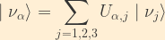
In general, relationship between the mass and flavour eigenstates is defined by a unitary matrix, U, by the following relationship:
Here, the 

Due to the unitarity of U (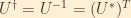
Neutrino Oscillation: Two Flavour Approximation
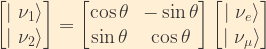
The weak eigenstates are related to the mass eigenstates by a simple unitary (length preserving) matrix:
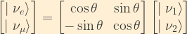
This matrix relationship is simply a more compact representation of the following two equations:


In other words, the weak eigenstates are coherent linear superpositions of the mass eigenstates. Here, 

Note that if the flavour eigenstates and mass eigenstates are equivalent, theta goes to zero, and the PMNS matrix simply becomes the Identity matrix.
This relationship can also be inverted to give the mass eigenstates as superpositions of the flavour eigenstates:
We assume that the mass eigenstates for the free neutrino as a function of time are simply plane waves:
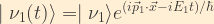

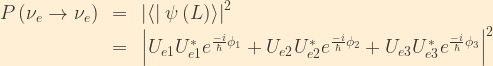
Suppose we have a weak decay producing an electron neutrino at time t=0. That neutrino expressed in terms of the mass eigenstates 


Combining this with the time-dependent representations of the mass eigenstates, and taking the direction of the neutrino’s motion to be along the z-axis, we see that the time evolution of the neutrino wavefunction is given by:
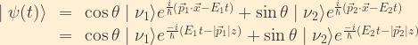
Now, looking at the beta particle energy distribution which prompted this whole neutrino business, we see that the peak is far from the cutoff (where the neutrino energy is zero), so, by and large, neutrinos are not “cold.” With their infinitesimally small mass, the bulk of the energy involved in neutrino production goes into their kinetic energy rather than rest mass. As a consequence, neutrinos can be expected to have velocities approaching (but not quite reaching) the speed of light in both the laboratory and center-of-mass reference frames. This assumption is born out by measurements of neutrino velocities performed in the wake of the OPERA “superluminal” neutrino fiasco, including those performed by the OPERA team once they found and corrected their hardware problem. So, for mathematical simplicity, we can make the very good assumption that 


Furthermore, we know from the energy-momentum relation from special relativity the following:


For the reasons discussed above, we may assume that 
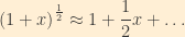


Therefore:
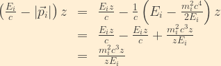
So, our expression for the wave function as a function of distance now becomes:

where 
Now, expressing the mass eigenstates in terms of the weak eigenstates:

Recall that I mentioned earlier that oscillation would not occur if the flavour eigenstates and mass eigenstates were identical. That becomes very clear in this expression. That equivalence would mean that 
Likewise, it is evident at this point if all of the neutrino eigenstates have identical masses, that would mean that 
If the masses are different, the wave function no longer remains purely an electron neutrino. We can calculate the probability of a flavour change by taking the projection of our wave function against the muon neutrino basis component and taking the absolute square:
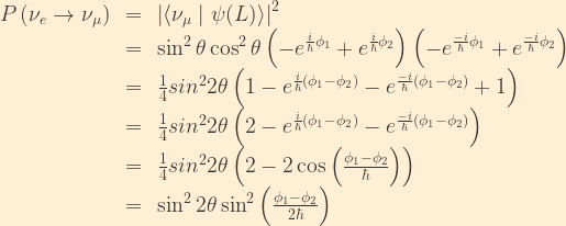
Where
(Yeah, I had to dredge up quite a few trig identities that I’ve not used in decades. Thank goodness for Wolfram Alpha.)
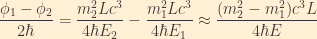
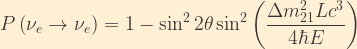
Thus we find that the two-flavour oscillation probability as a function of distance L is:
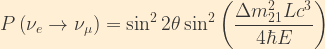
where
The two-flavour survival probability is then:
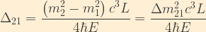
The wavelength for flavour oscillation is then given by:
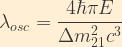
(A quick double-check of this result via dimensional analysis shows that this reduces to units of length. Wee!)
Neutrino Oscillation: Three Flavours
Extending what we have done to the case of three neutrino flavours is quite straightforward. In fact, we will be able to re-use quite a bit of the work we have already done.
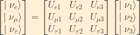
The matrix representation of the relationship between flavour and mass eigenstates is given by the following:
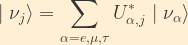
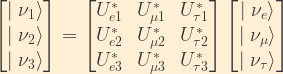
Due to the unitarity of the U matrix, this relationship can be inverted to represent mass eigenstates in terms of flavour eigenstates:
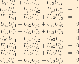
Now, since 
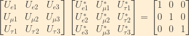
This encodes the following relationships, which will prove useful as we continue:
Now consider the case of an electron neutrino produced at t=0, propagating along the z axis.

The evolution of the wavefunction as a function of time is
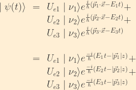
As before, we can make use of the assumptions that

where
Now, expressing the mass eigenstates in terms of the weak flavour eigenstates:
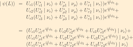
We can now calculate the probability for oscillation from an electron neutrino to a muon neutrino:

From the unitarity relations previously derived, remember that 
Now, from basic algebra on the complex plane, we know that 
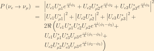
From the unitarity relations, we know that 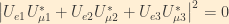

Substituting this back into our probability calculation gives the following:
![\displaystyle \begin{array}{rcl} P\left(\nu_e\rightarrow\nu_{\mu}\right) &=& 2\Re\left\{U_{e1}U_{\mu1}^*U_{e2}^*U_{\mu2}\left[e^{\frac{-i}{\hbar}\left(\phi_1 - \phi_2\right)}-1\right]\right\} +\\ &&2\Re\left\{U_{e1}U_{\mu1}^*U_{e3}^*U_{\mu3}\left[e^{\frac{-i}{\hbar}\left(\phi_1 - \phi_3\right)}-1\right]\right\} +\\ &&2\Re\left\{U_{e2}U_{\mu2}^*U_{e3}^*U_{\mu3}\left[e^{\frac{-i}{\hbar}\left(\phi_2 - \phi_3\right)}-1\right]\right\} \end{array}](https://s0.wp.com/latex.php?latex=%5Cdisplaystyle+%5Cbegin%7Barray%7D%7Brcl%7D++P%5Cleft%28%5Cnu_e%5Crightarrow%5Cnu_%7B%5Cmu%7D%5Cright%29+%26%3D%26+2%5CRe%5Cleft%5C%7BU_%7Be1%7DU_%7B%5Cmu1%7D%5E%2AU_%7Be2%7D%5E%2AU_%7B%5Cmu2%7D%5Cleft%5Be%5E%7B%5Cfrac%7B-i%7D%7B%5Chbar%7D%5Cleft%28%5Cphi_1+-+%5Cphi_2%5Cright%29%7D-1%5Cright%5D%5Cright%5C%7D+%2B%5C%5C++%26%262%5CRe%5Cleft%5C%7BU_%7Be1%7DU_%7B%5Cmu1%7D%5E%2AU_%7Be3%7D%5E%2AU_%7B%5Cmu3%7D%5Cleft%5Be%5E%7B%5Cfrac%7B-i%7D%7B%5Chbar%7D%5Cleft%28%5Cphi_1+-+%5Cphi_3%5Cright%29%7D-1%5Cright%5D%5Cright%5C%7D+%2B%5C%5C++%26%262%5CRe%5Cleft%5C%7BU_%7Be2%7DU_%7B%5Cmu2%7D%5E%2AU_%7Be3%7D%5E%2AU_%7B%5Cmu3%7D%5Cleft%5Be%5E%7B%5Cfrac%7B-i%7D%7B%5Chbar%7D%5Cleft%28%5Cphi_2+-+%5Cphi_3%5Cright%29%7D-1%5Cright%5D%5Cright%5C%7D+%5Cend%7Barray%7D&bg=FFEFD5&fg=333333&s=1&c=20201002)
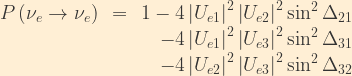
In a similar manner, we can calculate the electron neutrino survival probability:
We will now invoke the unitarity relationship 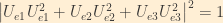
![\displaystyle \begin{array}{rcr} P\left(\nu_e\rightarrow\nu_e\right) &=& 1 + 2\left|U_{e1}\right|^2\left|U_{e2}\right|^2\Re\left[e^{\frac{-i}{\hbar}\left(\phi_1-\phi_2\right)}-1\right]\\ & & + 2\left|U_{e1}\right|^2\left|U_{e3}\right|^2\Re\left[e^{\frac{-i}{\hbar}\left(\phi_1-\phi_3\right)}-1\right]\\ & & + 2\left|U_{e2}\right|^2\left|U_{e3}\right|^2\Re\left[e^{\frac{-i}{\hbar}\left(\phi_2-\phi_3\right)}-1\right] \end{array}](https://s0.wp.com/latex.php?latex=%5Cdisplaystyle+%5Cbegin%7Barray%7D%7Brcr%7D++P%5Cleft%28%5Cnu_e%5Crightarrow%5Cnu_e%5Cright%29+%26%3D%26+1+%2B+2%5Cleft%7CU_%7Be1%7D%5Cright%7C%5E2%5Cleft%7CU_%7Be2%7D%5Cright%7C%5E2%5CRe%5Cleft%5Be%5E%7B%5Cfrac%7B-i%7D%7B%5Chbar%7D%5Cleft%28%5Cphi_1-%5Cphi_2%5Cright%29%7D-1%5Cright%5D%5C%5C++%26+%26+%2B+2%5Cleft%7CU_%7Be1%7D%5Cright%7C%5E2%5Cleft%7CU_%7Be3%7D%5Cright%7C%5E2%5CRe%5Cleft%5Be%5E%7B%5Cfrac%7B-i%7D%7B%5Chbar%7D%5Cleft%28%5Cphi_1-%5Cphi_3%5Cright%29%7D-1%5Cright%5D%5C%5C++%26+%26+%2B+2%5Cleft%7CU_%7Be2%7D%5Cright%7C%5E2%5Cleft%7CU_%7Be3%7D%5Cright%7C%5E2%5CRe%5Cleft%5Be%5E%7B%5Cfrac%7B-i%7D%7B%5Chbar%7D%5Cleft%28%5Cphi_2-%5Cphi_3%5Cright%29%7D-1%5Cright%5D+%5Cend%7Barray%7D&bg=FFEFD5&fg=333333&s=1&c=20201002)
We can simplify this expression by using the following relationship:
![\displaystyle \begin{array}{rcl} \Re\left[e^{\frac{-i}{\hbar}\left(\phi_1-\phi_2\right)}-1\right] &=& \cos{\left( \frac{\phi_2-\phi_1}{\hbar} \right)} - 1\\ &=& -2\sin^2{\frac{\phi_2-\phi_1}{2\hbar}}\\ &=& -2\sin^2{\frac{\left(m_2^2 - m_1^2\right)c^3L}{4\hbar E}} \end{array}](https://s0.wp.com/latex.php?latex=%5Cdisplaystyle+%5Cbegin%7Barray%7D%7Brcl%7D++%5CRe%5Cleft%5Be%5E%7B%5Cfrac%7B-i%7D%7B%5Chbar%7D%5Cleft%28%5Cphi_1-%5Cphi_2%5Cright%29%7D-1%5Cright%5D+%26%3D%26+%5Ccos%7B%5Cleft%28+%5Cfrac%7B%5Cphi_2-%5Cphi_1%7D%7B%5Chbar%7D+%5Cright%29%7D+-+1%5C%5C++%26%3D%26+-2%5Csin%5E2%7B%5Cfrac%7B%5Cphi_2-%5Cphi_1%7D%7B2%5Chbar%7D%7D%5C%5C++%26%3D%26+-2%5Csin%5E2%7B%5Cfrac%7B%5Cleft%28m_2%5E2+-+m_1%5E2%5Cright%29c%5E3L%7D%7B4%5Chbar+E%7D%7D++%5Cend%7Barray%7D&bg=FFEFD5&fg=333333&s=1&c=20201002)
Now, for the sake of convenience, let us define some shorthand notation:
where 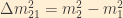
Here, 
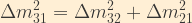
Given only three neutrino generations, there are only two independent mass-squared differences:
Discrete Symmetries in Weak Interactions
Consider for a moment time reversal symmetry, violation of which is mathematically equivalent to a CP violation. We can calculate the probability for a transition from a muon neutrino to an electron neutrino in the same manner in which we have previously calculated the opposite transition, or we can simply swap the relevant labels from the previous result:
![\displaystyle \begin{array}{rcl} P\left(\nu_{\mu}\rightarrow\nu_e\right) &=& 2\Re\left\{U_{\mu1}U_{e1}^*U_{\mu2}^*U_{e2}\left[e^{\frac{-i}{\hbar}\left(\phi_1 - \phi_2\right)}-1\right]\right\} +\\ &&2\Re\left\{U_{\mu1}U_{e1}^*U_{\mu3}^*U_{e3}\left[e^{\frac{-i}{\hbar}\left(\phi_1 - \phi_3\right)}-1\right]\right\} +\\ &&2\Re\left\{U_{\mu2}U_{e2}^*U_{\mu3}^*U_{e3}\left[e^{\frac{-i}{\hbar}\left(\phi_2 - \phi_3\right)}-1\right]\right\} \end{array}](https://s0.wp.com/latex.php?latex=%5Cdisplaystyle+%5Cbegin%7Barray%7D%7Brcl%7D++P%5Cleft%28%5Cnu_%7B%5Cmu%7D%5Crightarrow%5Cnu_e%5Cright%29+%26%3D%26+2%5CRe%5Cleft%5C%7BU_%7B%5Cmu1%7DU_%7Be1%7D%5E%2AU_%7B%5Cmu2%7D%5E%2AU_%7Be2%7D%5Cleft%5Be%5E%7B%5Cfrac%7B-i%7D%7B%5Chbar%7D%5Cleft%28%5Cphi_1+-+%5Cphi_2%5Cright%29%7D-1%5Cright%5D%5Cright%5C%7D+%2B%5C%5C++%26%262%5CRe%5Cleft%5C%7BU_%7B%5Cmu1%7DU_%7Be1%7D%5E%2AU_%7B%5Cmu3%7D%5E%2AU_%7Be3%7D%5Cleft%5Be%5E%7B%5Cfrac%7B-i%7D%7B%5Chbar%7D%5Cleft%28%5Cphi_1+-+%5Cphi_3%5Cright%29%7D-1%5Cright%5D%5Cright%5C%7D+%2B%5C%5C++%26%262%5CRe%5Cleft%5C%7BU_%7B%5Cmu2%7DU_%7Be2%7D%5E%2AU_%7B%5Cmu3%7D%5E%2AU_%7Be3%7D%5Cleft%5Be%5E%7B%5Cfrac%7B-i%7D%7B%5Chbar%7D%5Cleft%28%5Cphi_2+-+%5Cphi_3%5Cright%29%7D-1%5Cright%5D%5Cright%5C%7D+%5Cend%7Barray%7D&bg=FFEFD5&fg=333333&s=1&c=20201002)
There is something very important to note here. Unless all elements of the PMNS matrix are real, 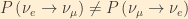
Consider the effects of the various symmetry operators:

We can’t include Parity or Charge Conjugation operators on their own because of the handedness issue. For example, C transforms left-handed neutrinos into left-handed anti-neutrinos, which, if they even exist, do not participate in weak interactions.
If weak interactions are invariant under CPT (which is generally assumed for ALL interactions):

If all of the PMNS matrix elements are not purely real:

So, if the PMNS matrix elements are not all real, CP is violated in neutrino oscillations, which would be an exiting result. (Exciting why? Well, that is a story for another day.) Unfortunately, current neutrino experiments lack the sensitivity to detect such violations, but future “neutrino factories” should shed light on this.
It is worth a brief detour here here to note that arguments similar to those shown here were used to predict the existence of the third generation of quarks (top and bottom quarks). The decay of quarks from one flavour to another is described by the CKM matrix, which is mathematically quite similar to the PMNS matrix. In 1973, in an effort to explain observed CP violations in kaon decay, Makoto Kobayashi and Toshihide Maskawa reasoned that the CKM matrix had to be a 3×3 matrix rather than a 2×2 matrix in order to accommodate the CP violations, hence the need to introduce a third generation of quarks. This prediction was later confirmed in 1985 by observation of the top quark at Fermilab.
- M. Kobayashi, T. Maskawa (1973). “CP-Violation in the Renormalizable Theory of Weak Interaction”.Progress of Theoretical Physics 49 (2): 652. Bibcode1973PThPh..49..652K. doi:10.1143/PTP.49.652.
- F. Abe et al. (CDF Collaboration) (1995). “Observation of Top Quark Production in pp Collisions with the Collider Detector at Fermilab”. Physical Review Letters 74 (14): 2626–2631. Bibcode1995PhRvL..74.2626A.doi:10.1103/PhysRevLett.74.2626. PMID 10057978.
- S. Abachi et al. (DØ Collaboration) (1995). “Search for High Mass Top Quark Production in pp Collisions at√s = 1.8 TeV”. Physical Review Letters 74 (13): 2422–2426. Bibcode 1995PhRvL..74.2422A.doi:10.1103/PhysRevLett.74.2422.
The Neutrino Mass Hierarchy
Right now, neutrino oscillation data allows us only to indirectly measure differences in the squares of the masses, not the masses themselves. Quite frankly, we don’t even know the order of the mass eigenstates from lightest to heaviest. We have two primary sources of neutrinos for these measurements (aside from reactors and accelerators): atmospheric neutrinos (produced by interactions between cosmic rays and the upper atmosphere), and solar neutrinos. These two sources provide two vastly different difference scales for benchmarking oscillation rates. In solar neutrinos, oscillation between the first and second mass eigenstates seems to be predominate, with 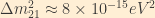

A new experiment called NOνA (which recently started collecting data) should be able to determine whether neutrinos have a normal mass hierarchy or inverted mass hierarchy.
The Parameterized PMNS Matrix
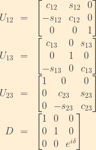
The elements of the PMNS matrix are usually expressed in a format in which they are parameterized in terms of three mixing angles, 


Let us now introduce some additional shorthand: 

The parameterized PMNS matrix is constructed as follows:
where
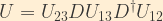
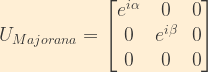
In the event that neutrinos prove to be Majorana fermions (in other words, neutrinos are their own anti-particles), there is an additional term which essentially adds two additional complex phases to the Dirac CP-violating phase:
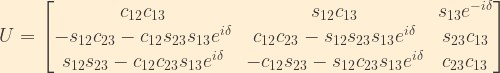
But, ignoring that for the moment, the parameterized PMNS matrix takes the following form when the above sub-matrices are multiplied out:

Pingback: Premio Nobel de Física 2015: Kajita (SuperKamiokande) y McDonald (SNO) por la oscilación de los neutrinos | Ciencia | La Ciencia de la Mula Francis