Before I dive into trying to explain Monday’s big announcement, I would like you to take a moment to watch this video showing Chao-Lin Kuo of Stanford University, the designer of the BICEP2 detector, revealing to Andrei Linde, one of the architects of inflationary cosmology, the big news. Seriously, take a look.

You can see Linde’s knees weaken when the news sinks in that his life’s work has been validated, bringing to mind the image of Peter Higgs wiping tears from his eyes on July 4, 2012 as the five-sigma discovery of his boson was announced at CERN. Linde’s wife, Renata Kallosh, also a physicist, was also visibly moved. She knew quite well how much this moment meant to him.

The Announcement

So what was this breakthrough that had such an impact on Linde and his wife, not to mention making cosmologists and astrophysicists around the world giddy with delight?

On Monday, March 17, 2014, the BICEP2 collaboration (an NSF-funded experiment jointly operated by Stanford/SLAC, the Harvard-Smithsonian Center for Astrophysics, Caltech JPL, UMN, and other institutions) announced the detection of primordial b-mode polarization in the Cosmic Microwave Background, consistent with the theoretically-predicted imprint of primordial gravitational waves amplified in scale by cosmological inflation.

“What?” I hear you cry.

Okay, time for me to back up a bit and try to put that into plain English.

But What Does It Mean?

But before I take a stab at explaining, take a look at this very quick and dirty explanation by Henry Reich over at MinutePhysics. When I try to explain this, I tend to gesture a lot. That doesn’t exactly come through in a blog post, so the animations in this video will have to serve in the place of such gestures.

In a similar vein, you might which to take a look at this comic explainer from PhD Comics.

So that’s the 30,000 foot view. Let’s start to zoom in a little bit. To do so, I’ll need to fill in a bit of background, making sure that we are all on the same page with definitions and concepts. (Bear with me for a bit, since there is a LOT of ground to cover.) So let’s start at the beginning. The VERY beginning.

The Big Bang (A Ridiculously Brief History)

A mere century ago, the accepted view of cosmology was pretty simple. As far as any astronomers new, our Milky Way Galaxy was the only galaxy there was, occupying a simple, static, relatively unchanging universe. Oh, sure, astronomers had long known “spiral nebulae,” and the 18th century philosopher Immanuel Kant had even speculated that they might be “island universes,” but astronomers had no good evidence that they actually lay beyond the bounds of our own Milky Way.

Then, in 1915, Einstein developed his general theory of relativity, which described gravity in terms of the curvature of space-time. However, it didn’t take long for it to become clear that his gravitational field equations on a cosmic scale could lead to only two solutions: an expanding universe or a contracting universe. To make his equations consistent with the prevailing idea of a static universe, he tweaked them by incorporating a “cosmological constant” term which allowed for a static solution.

Now, I have previously discussed how Henrietta Leavitt had, in 1908, discovered a correlation between the the intrinsic brightness and the periodicity of a certain class of variable stars known as Cepheid variables. By the 1920s, several astronomers, including Vesto Slipher, Gustaf Strömberg, and Edwin Hubble, had been using this relationship as a “yardstick” (along with other techniques) for measuring the distances to spiral nebulae. Not only had these measurements firmly established the fact that the spiral nebulae were, in fact, distinct galaxies a great distance beyond the Milky Way, but it was clear from comparing the distances with their redshift that they were, on average, moving away from us, and that the greater their distance, the faster they were moving. The universe was expanding, and Einstein’s cosmological constant was not needed!

As I’ve also previously written, Monsignor George Lemaître, a Belgian priest and astronomer, had studied these results, along with Einstein’s general relativity. By 1931, he had taken the facts at hand to their logical conclusion: further back in time, the universe was denser and hotter. This was the beginning of the Big Bang Theory of cosmology. That label was derisively coined in 1949 by the noted astronomer Sir Fred Hoyle, who stubbornly clung to the notion of a static universe in spite of the data.

Remember, boys and girls, evidence is the final arbitrator of reality, not the opinions of an authority figure, no matter how intelligent, highly-regarded, or accomplished they are. And all knowledge is provisional, subject to updates based upon new evidence. Even legendary intellects such as Einstein and Hoyle were wrong from time to time.

The Cosmic Microwave Background (CMB)

The statement in bold-face type in the previous section is the core of the Big Bang Theory. Filling in the details to form fully-fledged cosmological models has of course been the challenging part, with the construction of more and more detailed mathematical models and comparing them with observational data. One of the major predictions of big bang cosmology is that the very early universe was so hot and dense that it would have been permeated by plasma (ionized gas). This plasma would have been so dense that photons would not be able to travel through it very far before being scattered or absorbed by electrons or nuclei, thus rendering this early universe opaque. However, as the universe expanded and cooled, a point would eventually be reached at which electrons could finally bond to nuclei, allowing the material permeating space to transition to a neutral gas that is largely transparent to light. Cosmologists refer to this event as “recombination,” an event which is currently estimated as having taken place when the universe was a mere 378,000 years old. Once this transition took place, photons were then free to travel along their merry way, filling the universe with light. (Cosmologists often refer to the last vestiges of this cooling plasma as these photons bounced off of it for the last time as the “last scattering surface.” This concept figures prominently in the experimental results that we are building up to, so keep that in mind.)

The last scattering surface (also referred to as the cosmic photosphere) would have had a temperature in the neighborhood of 3000 K. Now, the radiation from an idealized thermal absorber and emitter (called a “black body“) will have a spectrum that is described by Planck’s law (or classically by the Rayleigh-Jeans law). While the peak of the spectrum from a 3000 K gas would be in the infrared, plenty of it would still be in the visible range. So why isn’t the light from the last scattering surface visible filling the night sky? Simply put, as the universe continued expanding, the wavelengths of this once bright light permeating the cosmos were then stretched out to longer wavelengths, dragging this primordial light into the long microwave portion of the spectrum.

For the benefit of those of you whose eyes just glazed over from that explanation, let me put it in terms that are a bit easier to grasp. Imagine a blacksmith pulling a chunk of iron from his forge after he’s gotten it seriously hot. It starts off glowing white hot, since the light emitted from it has components from across the entire visible spectrum. However, as the iron cools, it starts to glow red. The peak of the spectrum has shifted to the longer wavelengths. Eventually, it stops glowing in visible light, but is still hot to the touch. At this point, the light it is emitting is in the infrared spectrum. In other words, color correlates with temperature, and the light from recombination has, over the eons, shifted further into the infrared and into the microwave regions of the spectrum as the universe has expanded and cooled.

That is precisely where it was found in 1964 by Arno Penzias and Robert Wilson. The best current measurements of this cosmic microwave background (CMB) which they found filling the sky has a spectrum corresponding to a black body with a temperature of 2.7 K. The universe has cooled quite a bit in the 13.8 billion years which have elapsed since the recombination epoch.

Below is a graph of the CMB spectrum measured by the FIRAS instrument aboard the COBE satellite in the early 90s, overlayed upon the black body curve predicted by theory. The error bars are so tiny and the data points so closely match theory that the data points are indistinguishable from the theoretical curve in this graph (thus serving as the inspiration for this xkcd comic).

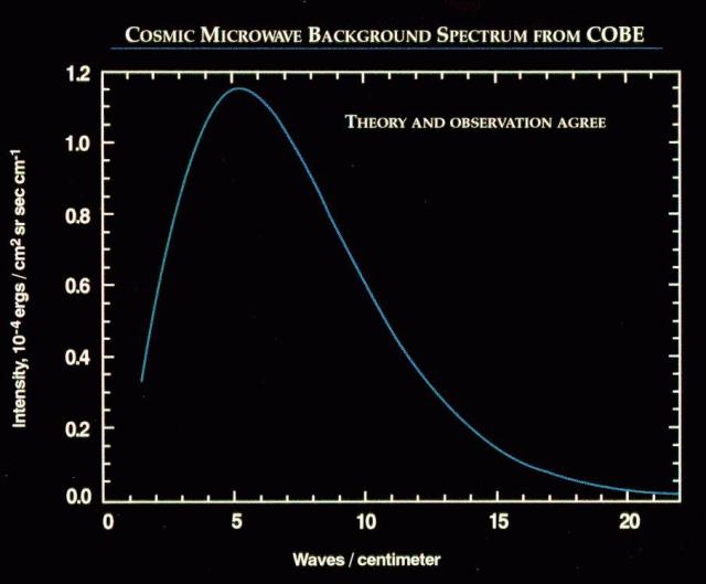
FIRAS/COBE CMB spectrum overlayed upon black body spectrum predicted by theory.
Image courtesy of NASA.

Inflation

One thing that quickly became apparent in the early days of studying the CMB was just how incredibly uniform it is. No matter where one looks in the sky, the CMB has the same temperature. (That said, there are TINY fluctuations in the CMB, on the order of micro-Kelvins, and those are critical to this entire discussion, but we’ll get to them shortly.) This had cosmologists somewhat baffled. After all, how could portions of the CMB on opposite sides of the sky, which had never been in proximity with one another long enough to reach thermal equilibrium, be the same temperature?

In the mid- to late-1970s, Alan Guth was trying to figure out why magnetic monopoles had never been observed, despite being predicted by several attempts at unifying the fundamental forces of nature. He was working with some ideas about “cosmic phase transitions” pioneered earlier in that decade by Andre Linde (the gentleman from the video earlier), and, on December 7, 1979, had what he described in his notebook as “a spectacular realization.” He realized that a period of exceedingly fast expansion of spacetime in the early universe (inflation) many orders of magnitude more rapid than the currently-observed expansion would not only fix the monopole problem, but would also address the overall uniformity of the CMB, as well as taking care of an old cosmological problem described by Robert Dicke in 1968 as the “flatness problem.” The math worked out beautifully for addressing all of these issues. Guth’s model was not without its own problems, however. In the early 1980s, Linde refined Guth’s model, molding it into the modern model of cosmic inflation.

Assuming that inflation proves to be correct, the underlying scalar inflaton field which would have driven it remains one of the remaining gaps in the standard model of particle physics, along with a quantum description of gravity (more on that in a moment, as the results we are building up to have bearing on that subject), grand unification of the strong and electroweak gauge forces, neutrino mass, the hierarchy problem, and an explanation for dark energy and dark matter (not to be confused with one another). Those are the major blank spots on our map of knowledge of physics. Here there be dragons.

The History of the Universe (Image courtesy of BICEP/KECK)

Precision Measurements of the CMB

Although inflationary cosmology was originally inspired by the observed uniformity of the CMB, inflation theory actually predicts that there should actually be a certain degree of non-uniformity of the CMB, in the form of extremely tiny fluctuations in the temperature. By tiny, I mean millionths of Kelvin. These irregularities would be caused by rapid inflation magnifying tiny quantum fluctuations to macroscopic scales, resulting in slight variations in the density of the last scattering surface. (Remember the last scattering surface? We’ll be returning to it again.)

Over the years, we’ve managed to build more and more sensitive instruments for detecting such fluctuations, and they are in fact there:

COsmic Background Explorer (COBE) 1992

COBE map of the CMB
Image courtesy of NASA

Wilkinson Microwave Anisotropy Probe (WMAP) 2003

WMAP map of the CMB
Image courtesy of NASA

Planck 2013

Planck map of the CMB
Image courtesy of NASA

As it turns out, the Planck results represent the highest resolution image we can ever get of the CMB. Here, we are not bumping into the limits of the technology, but rather an inherent fuzziness in the data caused by the long wavelengths which are being observed. But mapping these temperature fluctuations is not the only thing Planck was designed to detect. It was also design to collect information about the polarization of the CMB, which is at the heart of Monday’s announcement. But the BICEP2 team beat the Planck team to the punch. The Planck data is still being analyzed, and it will be very interesting to see the results of that analysis in comparison with the BICEP2 results. (Remember, reproduction of results is a critical part of the scientific method.)

In any case, the data collected by COBE, WMAP, and Planck have been a treasure trove for cosmologists and astrophysicists. This data has helped with refining estimates of the age of the universe, the proportions of normal baryonic matter, dark matter, and dark energy, refining estimates of Hubble’s constant, and estimating the overall curvature of spacetime on cosmic scales. (The visible universe appears to be roughly flat, which is consistent with inflationary theory.) This data has even been used to place constraints on neutrino mass and the number of neutrino flavors (there are three, and Planck backs that up), and even constraining various proposed models for dark matter.

One would not naively expect all of those speckles in the images above to yield so much useful information, but scientists have plenty of ways of slicing and dicing the data in useful ways. For example, just as an audio engineer can decompose a sound signal into a spectrum showing the strength each component frequency (by taking a Fourier transform), astrophysicists can decompose the CMB data in terms of something called spherical harmonics (the same mathematical constructs used to describe the quantum probability wave of an electron in an atom) to produce an angular power spectrum. Such a power spectrum shows the intensity of the fluctuations as a function of their angular size. And in that analysis lies a wealth of useful information.

One consequence of these density fluctuations in the early universe is that the matter that would go on to form the galaxies would be expected to be distributed through the universe in web of filaments. Computer simulations of the evolution of the large scale structure of the universe based upon this assumption are consistent with what is actually observed. Compare, for example, the Millennium Simulation with the results of the Sloan Digital Sky Survey and the 2dF Galaxy Redshift Survey.

Polarization

Stay with me. We are almost there. We have just a few more fundamental concepts to go over before we get to the big show.

A Tale of Two Modes

The two polarization modes expected in the CMB are derived by applying Helmholtz decomposition (a.k.a., the fundamental theorem of vector calculus) to the vector field describing the polarizations. Using this decomposition, such a vector field can be described as the sum of two components, a curl-free component and a divergence-free component.

If $\displaystyle \kappa$ is the density field producing the polarization, and $\displaystyle \vec{u}$ is the resulting polarization vector any any given point in the vector field, we may observe that $\displaystyle \nabla\kappa = \vec{u}$ . Separating the density field into the aforementioned components, we obtain:

$\displaystyle \nabla^2\kappa^E = \nabla\cdot\vec{u}$ , $\displaystyle \nabla^2\kappa^E = \nabla\times\vec{u}$

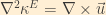
Here, we are using the label E to denote a scaler potential component by analogy with an electric field, and B to denote the vector potential component by analogy with a magnetic field.

This is as good of a time as any to discuss polarization. The main contexts in which you’ve likely been exposed to this concept is in terms of polarizing sunglasses and 3D movies. Light, as described by classical electrodynamics, consists of an electric field oscillating at right angles to a magnetic field, with both fields oscillating at right angles to the direction in which the light is traveling. Most thermal (heat-based) light sources emit light that has those fields pointing at a mix of random angles (but still perpendicular to the direction the light is travelling). However, if the light passes through a polarizing filter, which blocks all light except that which has the electric field oscillating in a certain direction, we have what is called linearly polarized light. (There is also another mode of polarization called circular polarization, where the direction that the electric field is pointing follows a corkscrew path as the light travels. That is what is used with 3D movie glasses.)

But another way to get linear polarization of the light is for it to bounce, or “scatter” off of something. Light that has been scattered through the atmosphere or bounced off of water or glass is generally horizontally polarized, which is why polarizing sunglasses are able to cut glare. This process of light getting polarized by bouncing off of something is particularly strong when the matter scattering the light is charged, via a process called Thomson scattering (first explained by J. J. Thomson, the discoverer of the electron).

Recall that I earlier mentioned that the plasma cooling to neutral gas during the recombination epoch is sometimes referred to as the “last scattering surface.” Because of Thomson scattering from this last bit of plasma from the earlier universe, the microwaves from the CMB are polarized, and encoded in the patterns of that polarization (with respect to the fluctuations in the CMB) is information about how the last scattering surface was moving at the time that the light last bounced off of it.

Those patterns of polarization can be mathematically analyzed and broken down into two independent modes: E-mode polarization and B-mode polarization. (The names come from analogy with the vector behavior of electric (E) and magnetic (B) fields in classical electrodynamics. (For a slightly more technical treatment, see sidebar: “A Tale of Two Modes.”) E-mode polarization, which is the more straightforward type, should be either directly parallel to or perpendicular to the boundaries of temperature fluctuations in the CMB. B-mode polarization, which would manifest as being at angles across those boundaries, can be caused by one of two things: gravitational lensing of E-mode polarization, or the presence of gravitational waves in the last scattering surface.

Gravitational Waves

That’s right, gravitational waves, subtle fluctuations in the fabric of spacetime. They are really the last remaining unverified major prediction of general relativity. We are pretty sure from indirect evidence that they exist, based upon studies of the orbital decay of Hulse-Taylor binary pulsars (pairs of neutron stars orbiting one another), but they have yet to be directly detected. There are efforts to detect gravitational waves underway or under construction, but it is an amazingly difficult task. Imagine using a 2-mile long interferometer to try to detect a brief change in the length of that apparatus of less than the diameter of a proton. Yeah, that difficult.

But if indications of primordial gravitational waves (which had been amplified to tremendous scales by inflation) can be detected, it would be a tremendous feather in the cap for both general relativity and for inflation theory. After all, Linde actually predicted that such indications would be there decades ago. What’s more, such indications could also be taken as a hint of quantum gravity, since the initial fluctuations (prior to being amplified by inflation) would have been at the quantum scale. Proving the quantum nature of gravity (or that it even IS quantum in nature, as opposed to an emergent pseudo-force as described by general relativity) has long been a challenge. Thus far, efforts at constructing a quantum theory of gravitation have tended to result in mathematical divergences which have stymied generations of physicists.

The challenge here isn’t in detecting E-mode polarization or B-mode polarization, or in sorting them out from each other. Those things have been done before. E-mode polarization of the CMB was detected by DASI in 2002, and B-mode polarization was detected by the South Pole Telescope in 2013. The trick here is in sorting out the two possible sources of B-mode polarization. That means mapping out sources of gravitational lensing, and using that information to filter out the type of b-mode polarization that is not of interest, just leaving the primordial b-mode polarization due to gravitational waves.

The Breakthrough

Whew! Okay, we’re there. With that crash course in cosmology out of the way (without even bothering to take a detour into the strange topics of dark energy and dark matter), we are finally ready to talk about the big announcement.

The Dark Sector Lab (DSL), located 3/4 of a mile from the Geographic South Pole, houses the BICEP2 telescope (left) and the South Pole Telescope (right). (Steffen Richter, Harvard University, via BICEP/KECK.)

Officially, BICEP doesn’t stand for anything; but, unofficially, it stands for “Background Imaging of Cosmic Extragalactic Polarization,” and this is the team that beat Planck to the release of b-mode polarization data. The BICEP2 telescope, located at the Dark Sector Lab at the Amundsen-Scott South Pole Station, collected polarization data that was used to generate the following graph showing primordial b-mode polarization for a small patch of sky:

B-mode pattern observed with the BICEP2 telescope, with the line segments showing the polarization from different spots on the sky. The red and blue shading shows the degree of clockwise and anti-clockwise twisting of this B-mode pattern. (Image courtesy of BICEP/KECK.)

Of course, that graph doesn’t mean a great deal without a little interpretation. It is the twisty bits that are of interest. What it means is that primordial b-mode polarization has definitely been found.

For the more technically inclined, the value of r, the ratio of tensor to scalar amplitudes, comes out to 0.2, right in line with predictions from Linde, yet, strangely at odds with constraints placed on r by Planck results released thus far. (This means that it will be even more interesting to see what the final analysis of the Planck data reveals when it finally comes out.) The data also indicates that the energy scale for the inflation process is about 2×1016 GeV (close to the Planck scale of 2×1018 GeV).

What It Means

Of course, ultimately, these results will have to be validated by independent data, such as from the Planck Collaboration or elsewhere. As cosmologists Neil Turok points out, we shouldn’t jump to too many conclusions based upon this initial announcement.

But, if further data comes out from other teams backing up the BICEP2 results, here is a summary of the ramifications:

Strong, although still indirect, evidence supporting cosmological inflation
New bounds placed upon proposed inflaton models
New bounds on the energy scale of the inflationary epoch
Strong, although still indirect, evidence for gravitational waves
Hints at quantum gravity
A strong prospect for an eventual Nobel Prize for Guth and Linde

Of course, what it will really mean is that Stephen Hawking will have won a bet with Neil Turok.

BICEP2 Takes a Peek at Cosmic Inflation

The Announcement

But What Does It Mean?

The Big Bang (A Ridiculously Brief History)

The Cosmic Microwave Background (CMB)

Inflation

Precision Measurements of the CMB

Polarization

A Tale of Two Modes

Gravitational Waves

The Breakthrough

What It Means

For More Information

About Glen Mark Martin

1 Response to BICEP2 Takes a Peek at Cosmic Inflation

Leave a comment Cancel reply

Glen Mark Martin

Blog

Meta

Archives

Spyglass’ Ramblings

BICEP2 Takes a Peek at Cosmic Inflation

The Announcement

But What Does It Mean?

The Big Bang (A Ridiculously Brief History)

The Cosmic Microwave Background (CMB)

Inflation

Precision Measurements of the CMB

Polarization

A Tale of Two Modes

Gravitational Waves

The Breakthrough

What It Means

For More Information

Share this:

Related

About Glen Mark Martin

1 Response to BICEP2 Takes a Peek at Cosmic Inflation

Leave a comment Cancel reply

Glen Mark Martin

Blog

Meta

Archives

Spyglass’ Ramblings